


Introduction
Hello there, fellow learners! Welcome back to the 10th episode of our machine-learning adventure. As you might recall, we are exploring the fascinating world of logistic regression. In today's discussion, we will focus on the "cost function", an essential component of our learning journey.
Even though the term "cost function" may sound intimidating, don't worry! We are here to guide you through it and make it your new best friend. Think of it like a GPS for our model, helping it improve with each step. In this episode, we will avoid using complicated jargon and instead focus on what makes the cost function work.
Whether you are a coding expert or just beginning to understand the world of machine learning, we've got you covered. So, sit back and relax, and let us discover the secrets of the cost function together. Are you ready? Let's go! 🚀
Previous Episode Overview
In our previous episodes, we learned about logistic regression and its usefulness in solving classification problems. We explored the sigmoid function and gained a mathematical intuition of how it works. With each episode, we have come closer to mastering the skill of predictive modeling.
Purpose of Cost Function:
Let's dive into the purpose of the cost function. It works alongside our logistic regression model to improve the accuracy of our predictions.
1. Bridging the Gap: Imagine our model is on a quest to make predictions. It takes a swing, makes a guess, and then reality hits — it's not always spot on. The cost function steps in to measure the gap between our prediction and what happened. It's like a friendly referee saying, "Here's how close or far off you were, buddy."
2. Learning from Mistakes: The cool part? The cost function doesn't just point out mistakes; it helps our model learn from them. It nudges the model in the right direction, saying, "Hey, try adjusting this a bit and see if you can get closer next time." It's all about getting smarter with each prediction, like a self-improvement plan for our model.
3. Finding the Sweet Spot: Our ultimate goal? Minimize that gap. The cost function guides our model through this process of trial and error, helping it find the sweet spot where predictions align as closely as possible with reality. The secret sauce turns a good model into a great one.
How Cost Function Work?
Cost Function
Remember that the cost function allows you to measure how well a specific set of parameters fits the training data. Thereby, it gives you a way to try to choose better parameters. In this section, we'll look at how the squared error cost function is not an ideal cost function for logistic regression. We'll take a look at a different cost function that can help us choose better parameters for logistic regression. Here's what the training set for our logistic regression model might look like.
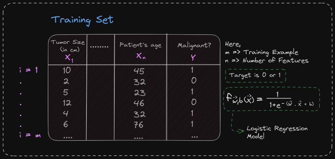
Here's what the training set for our logistic regression model might look like. Here each row might correspond to patients who were paying a visit to the doctor and one dealt with some diagnosis. As before, we'll use m to denote the number of training examples. Each training example has one or more features, such as the tumor size, the patient's age, and so on for a total of n features. Let's call the features X_1 through X_n. Since this is a binary classification task, the target label y takes on only two values, either 0 or 1. Finally, the logistic regression model is defined by this equation. The question you want to answer is, given this training set, how can you choose parameters w and b?
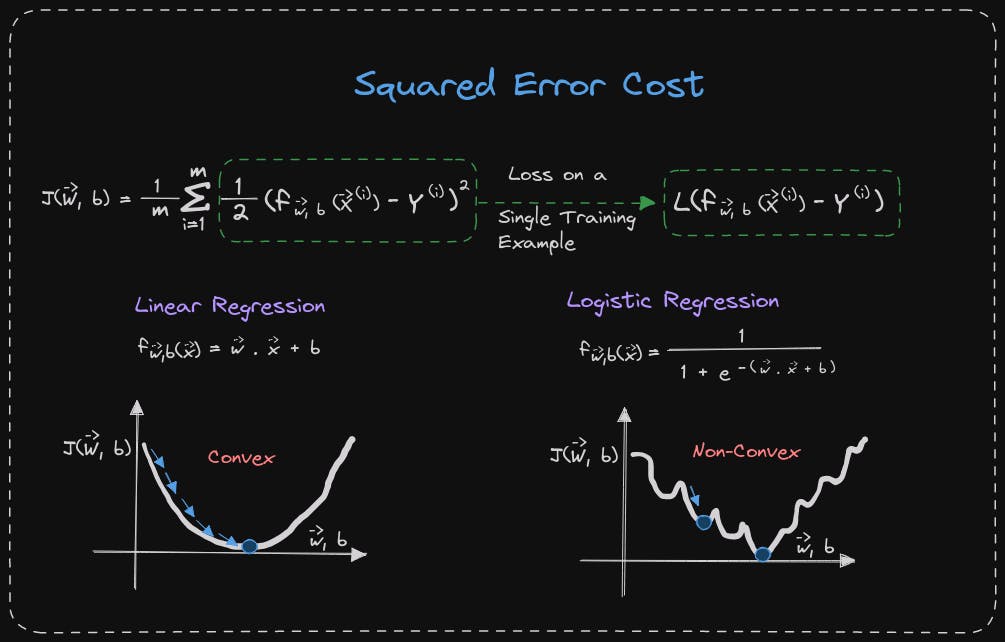
Recall for linear regression that the cost function is the squared error. The only difference is that the 1/2 has been moved inside the summation. In the case of linear regression, where f(x) is the linear function, w.x+b, the cost function is convex and has a bowl or hammer shape. Gradient descent will converge at the global minimum by taking one step at a time.
The same cost function cannot be used for logistic regression as the function becomes non-convex. If f(x) is defined as 1/(1+e^(-wx+b)), then the cost function will not be convex. This means that using gradient descent can result in getting stuck in local minima. Therefore, a different cost function should be used for logistic regression that can guarantee convergence to the global minimum.
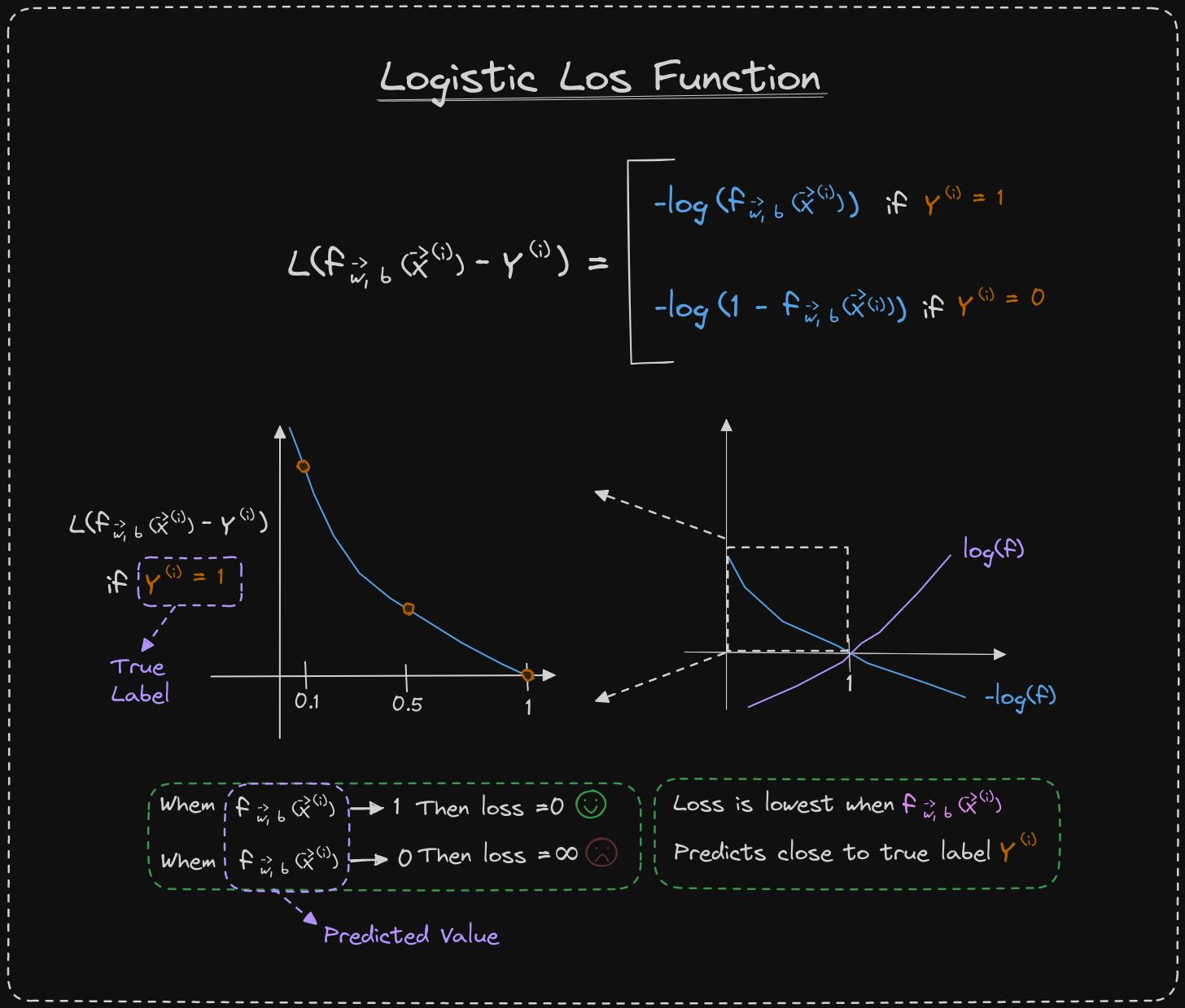
I have written down the definition of the loss function that we will use for logistic regression. If the label y equals 1, then the loss is the negative log of f of x. If the label y is equal to 0, then the loss is the negative log of 1 minus f of x. The loss function measures how well you are doing on one training example and sums up the losses on all of the training examples to get the cost function, which measures how well you are doing on the entire training set.
When y equals 1, the loss function incentivizes the algorithm to make more accurate predictions because the loss is lowest when it predicts values close to 1. If the algorithm predicts a probability close to 1 and the true label is 1, then the loss is very small, almost 0, because it is very close to the right answer.
On the other hand, if the algorithm predicts 0.5 and the true label is 1, then the loss is a bit higher but not too high. However, if the algorithm predicts 0.1 and the true label is 1, then the loss is much higher. Therefore, the loss function helps push the algorithm to make more accurate predictions when the true label is 1.
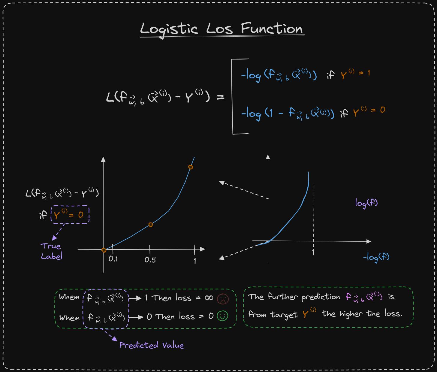
Let's examine the second part of the loss function, which corresponds to the scenario where y equals 0. In this case, the loss is the negative logarithm of 1 minus f of x. The graph of the function looks like a downward curve. The range of f is between 0 and 1 because logistic regression only outputs values within that range. If we zoom in, we can see that the vertical axis represents the value of the loss for different values of f of x. When f is 0 or close to 0, the loss is low. This means that if the true label is 0 and the model's prediction is close to 0, then the loss is appropriately low. However, as the value of f of x increases, the loss increases too, because the prediction becomes further from the true label 0. In fact, as the prediction approaches 1, the loss tends towards infinity.
Let's consider the example of tumor prediction. If the model predicts with 99.9 percent certainty that a patient's tumor is malignant, but it turns out to be benign (y equals 0), then the model is penalized with a very high loss. This high loss reflects the error in the model's prediction.
In the case where y equals 1, the further the prediction f of x is from the true value of y, the higher the loss. In fact, if f of x approaches 0, the loss tends towards infinity. Therefore, when the true label is 1, the model is motivated to not predict values too close to 0.
In the Section, we learned why the squared error cost function is not effective for logistic regression. Instead, we came up with a new definition for the loss function for logistic regression, which is used for a single training example. With this loss function, the overall cost function becomes convex. This means that gradient descent can be reliably used to find the global minimum. Although proving that this function is convex is beyond the scope of this section, we know that the cost function is a function of the entire training set. It is the average of the loss function on individual training examples. The cost is equal to 1 over m times the sum of all the training examples of the loss on the training examples. If you can find the value of the parameters, w and b, that minimizes this cost, you'd have a good set of values for the parameters w and b for logistic regression.
In the optional lab, you'll see why the squared error cost function is not effective for classification.
Optional Lab Link: Click Here
Simplified Cost Function For Logistic Regression
In this section, you will learn a simpler way to write the loss and cost functions for logistic regression. This will make the implementation of gradient descent easier when fitting the parameters of the model.
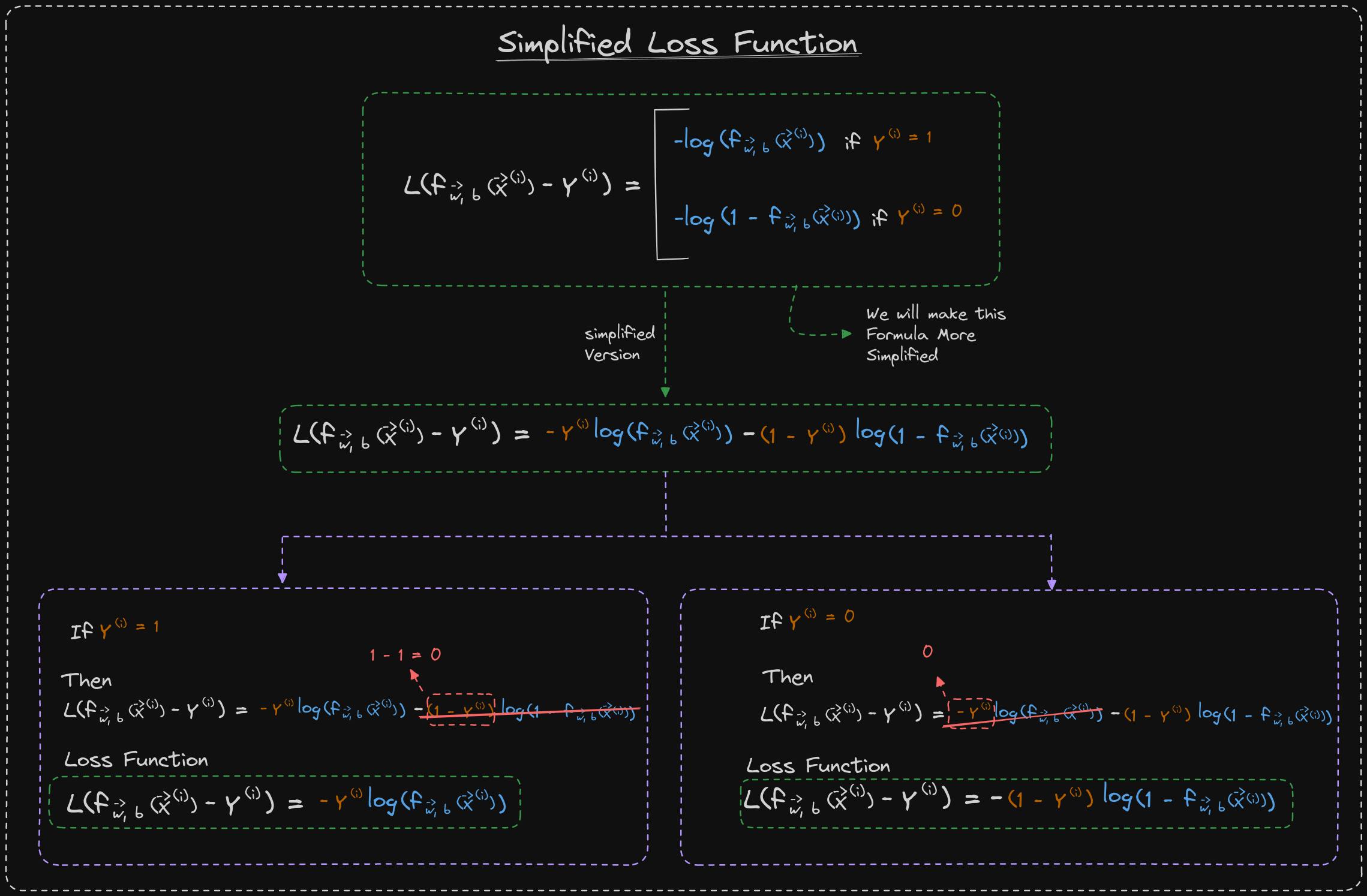
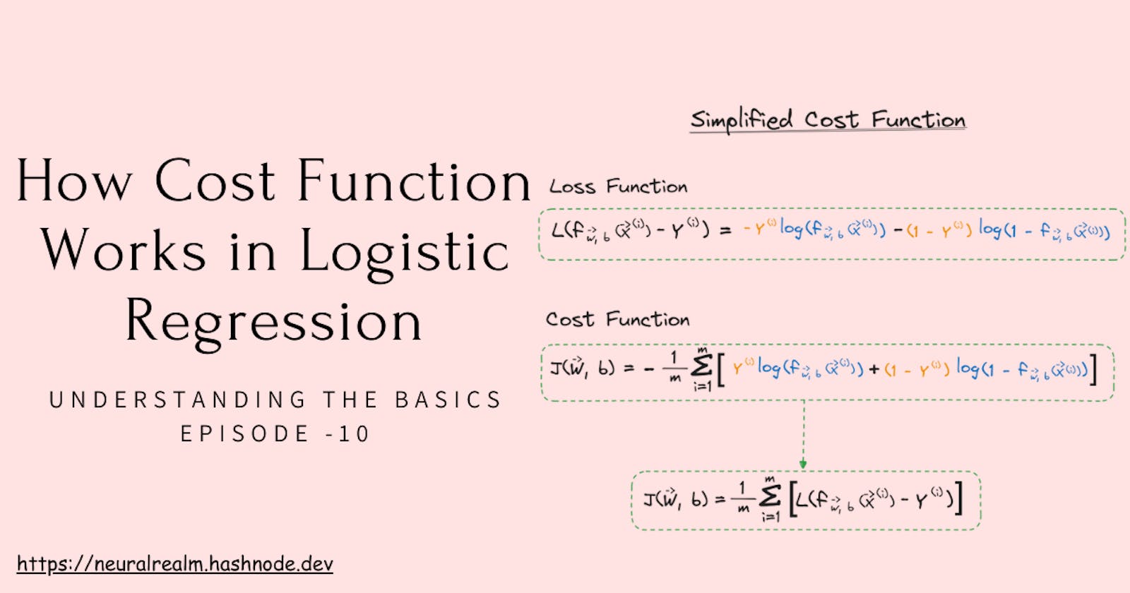
First, let's recall the loss function we defined in the previous video for binary classification problems, where y can only take on the values of zero or one. We can simplify this loss function to:
Loss = -y*log(f) - (1-y)*log(1-f)
This is equivalent to the more complex formula that we previously defined. To understand why, consider the two cases of y = 0 and y = 1.
If y = 1, then the second term (1-y)*log(1-f) becomes zero, and the loss function is just -log(f), which is the first term in the original loss function.
If y = 0, then the first term -y*log(f) becomes zero, and the loss function is just -log(1-f), which is the second term in the original loss function.
Therefore, this simplified loss function is equivalent to the original one, and it is easier to work with because it does not require separating the two cases of y = 0 and y = 1.
Using this simplified loss function, we can now write out the cost function for logistic regression.
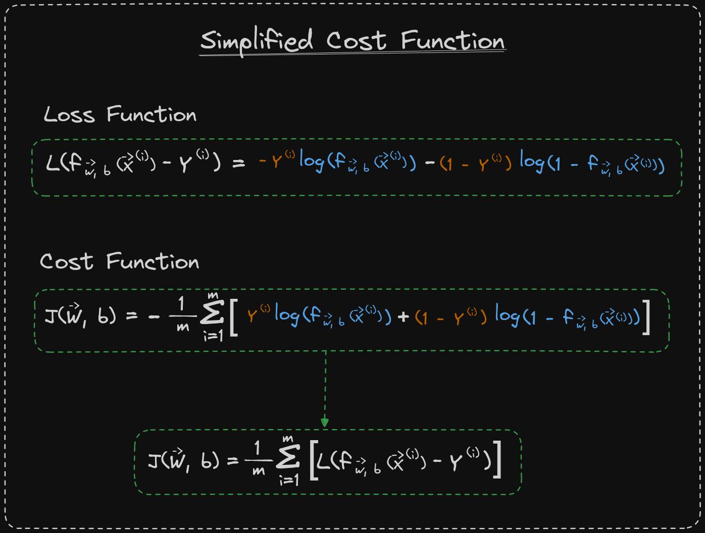
Let's recall that the cost J is calculated by averaging the loss across the entire training set of m examples. Mathematically, it can be represented as 1/n times the sum of loss from i equals 1 to m. If we substitute the definition for the simplified loss from above, then the expression for J becomes 1/m times the sum of the term above. By bringing the negative signs and moving them outside, we can simplify it further to derive the cost function. This cost function is widely used to train logistic regression.
You may be wondering why we have selected this particular function among numerous other cost functions. While we won't have the time to delve into the details of this episode, I'd like to mention that this specific cost function is derived from statistics, using the statistical principle of maximum likelihood estimation. This principle is a statistical approach to efficiently finding parameters for different models. The beauty of this cost function is that it is convex. However, don't worry about getting into the nitty-gritty of maximum likelihood, as it is merely a deeper rationale and justification behind our selection of this particular cost function.
The Practical lab will show you how the logistic cost function is implemented in code.
Practical Lab Link: Go to the Practical Link
🎙️ Message for Next Episode:
Now that we have simplified the cost function, we can proceed with applying gradient descent to logistic regression. in the next episode.
Resources For Further Research
Coursera - Machine Learning Specialization
This Article is heavily inspired by this Course so I will also recommend you to check this course out, there is an option to watch the
course for freeor you can buy the course to gain aSpecialization Certificate.Optional labs provided in this article are from this course itself.
"Hands-On Machine Learning with Scikit-Learn, Keras, and TensorFlow" by Aurélien Géron:
- A practical guide covering various machine learning concepts and implementations.
By the way…
Call to action
Hi, Everydaycodings— I’m building a newsletter that covers deep topics in the space of engineering. If that sounds interesting, subscribe and don’t miss anything. If you have some thoughts you’d like to share or a topic suggestion, reach out to me via LinkedIn or X(Twitter).
References
And if you’re interested in diving deeper into these concepts, here are some great starting points:
Kaggle Stories - Each episode of Kaggle Stories takes you on a journey behind the scenes of a Kaggle notebook project, breaking down tech stuff into simple stories.
Machine Learning - This series covers ML fundamentals & techniques to apply ML to solve real-world problems using Python & real datasets while highlighting best practices & limits.