


Welcome back! In the previous episodes, we learned about Linear Regression, a powerful tool for predicting continuous outcomes. We learned how to draw the best-fitting line through our data by optimizing parameters to minimize the difference between predicted and actual values.
Introduction
Logistic Regression: Simplifying Binary Classification
Logistic Regression is a core machine learning algorithm designed for binary classification tasks. Unlike Linear Regression, which predicts continuous outcomes, Logistic Regression focuses on situations where the goal is to categorize instances into one of two classes.
Key Features:
Binary Outcome:
- Suited for scenarios with two possible outcomes, such as spam or non-spam emails, customer churn, or disease presence.
Sigmoid Function:
- Utilizes the Sigmoid function to transform a linear combination of features into probabilities between 0 and 1.
Probability Threshold:
- Sets a threshold to convert probabilities into binary outcomes, determining class labels.
Log Odds and Odds Ratio:
- Outputs log odds, offering insights into the likelihood of an event, expressed as odds ratios.
Applications:
Medical Diagnosis: Predicting the presence of a medical condition.
Finance: Assessing loan default or detecting fraudulent transactions.
Marketing: Predicting customer churn or campaign response.
Social Sciences: Analyzing factors influencing binary outcomes in research.
Basics of Logistic Regression
In this episode, we'll unravel the fundamentals of Logistic Regression, a powerful algorithm tailored for binary classification tasks. Unlike Linear Regression, which predicts continuous outcomes, Logistic Regression is adept at handling scenarios where the goal is to categorize instances into one of two classes.
Binary Outcome
Logistic Regression is ideal when dealing with a binary outcome, where there are only two possible classes. Examples include spam or non-spam emails, customer churn (yes or no), and medical diagnosis (presence or absence of a condition).
Sigmoid Function
At the core of Logistic Regression is the Sigmoid function, also known as the logistic function. This mathematical curve transforms a linear combination of input features into probabilities. It squashes the output values between 0 and 1, making them interpretable as probabilities.
Probability Threshold
Unlike Linear Regression, Logistic Regression doesn't directly provide class labels. Instead, it produces probabilities. A threshold is set to convert these probabilities into binary outcomes. For example, if the probability is greater than 0.5, the instance is classified as the positive class; otherwise, it's classified as the negative class.
Learn From Scratch
Introduction
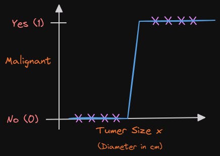
To explain how Logistic Regression works, let's take the example of determining whether a tumor is malignant. We assign the label '1' or 'yes' to positive cases (malignant tumors) and '0' or 'no' to negative cases (benign tumors). To represent the dataset in a graph, we plot the tumor size on the horizontal axis and only 0 and 1 values on the vertical axis since it is a classification problem. Using logistic regression, we can fit an S-shaped curve to the dataset.
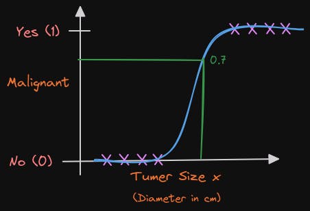
For this example, if a patient comes in with a tumor of this size, which I'm showing on the x-axis, then the algorithm will output 0.7 suggesting that is closer or maybe more likely to be malignant and benign. Will say more later what 0.7 actually means in this context. But the output label y is never 0.7 is only ever 0 or 1. To build out the logistic regression algorithm, there's an important mathematical function I like to describe which is called the Sigmoid function, sometimes also referred to as the logistic function.
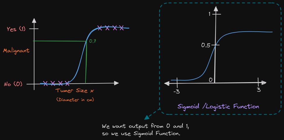
The Sigmoid function has a distinct shape, which is important to understand. The graph on the left represents tumor size on the x-axis, with only positive numbers. On the other hand, the graph on the right has a horizontal axis labeled Z, ranging from -3 to + 3 including negative and positive values. The Sigmoid function outputs a value between 0 and 1.
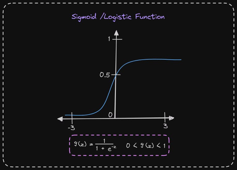
If we use g of z to denote a function, then the formula of g of z is equal to 1 over 1 plus e to the negative z. Here, e is a mathematical constant that has a value of approximately 2.7, and e to the negative z is e to the power of negative z. It's worth noting that if z were to be a large number, such as 100, e to the negative z would be e to the negative 100, which is tiny. Thus, g of z is 1 over 1 plus a tiny number, making the denominator close to 1. Consequently, when z is large, g of z, which is a Sigmoid function of z, is very close to 1. Similarly, when z is a very large negative number, g of z becomes 1 over a giant number, causing g of z to be close to 0. This explains why the sigmoid function has a shape that starts close to zero and gradually increases to the value of one.
Moreover, in the Sigmoid function, when z equals 0, e to the negative z is e to the negative 0, which equals 1, making g of z 1 over 1 plus 1, which equals 0.5. Therefore, the Sigmoid function passes the vertical axis at 0.5. This information helps us build up the logistic regression algorithm.
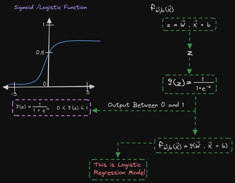
Let's go through the process of building up to the logistic regression algorithm step by step. In the first step, we define a straight line function as w multiplied by x plus b, similar to a linear regression function. We'll call this value z. Then, we pass this value of z to the Sigmoid function, also known as the logistic function, g. The formula for g of z is 1 over 1 plus e to the negative z. This output value lies between 0 and 1.
Now, when we combine the two equations, we get the logistic regression model f of x, which is equal to g of wx plus b, or g of z. Essentially, this model takes in a set of features X as input and outputs a number between 0 and 1.
Interpretation of Logistic Regression Output
Let's review how to interpret the output of logistic regression. We'll revisit the example of tumor classification. Think of logistic regression's output as the probability that the class or label y will be 1, given input x. For instance, in this application, where x is the size of the tumor, and y is either 0 or 1, if a patient has a tumor of a certain size x, and the model outputs x plus 0.7, then that means the model is predicting a 70 percent chance that the label y will be equal to 1 for this patient. In other words, the model is saying that the patient has a 70 percent chance of having a malignant tumor.
Now, let me ask you a question. If the chance of y being 1 is 70 percent, what is the chance that it is 0? Since y can only be 0 or 1, the probability of these two numbers must add up to 1 or 100 percent. Therefore, if the chance of y being 1 is 0.7 or 70 percent, then the chance of it being 0 must be 0.3 or 30 percent.
To gain a better understanding of how this process works, I recommend referring to this Notebook: Sigmoid Function Notebook
Decision Boundary
Suppose you want to learn an algorithm to predict the value of y, whether it's going to be zero or one. One way to do this is by setting a threshold above which you predict y to be one and below which you predict y to be zero. Typically, people choose a threshold of 0.5, which means if the value of f(x) is greater than or equal to 0.5, then you predict y to be one. This is denoted as y hat equals 1. On the other hand, if the value of f(x) is less than 0.5, then you predict y to be zero, which is denoted as y hat equals 0.
Now, let's dive deeper into when the model would predict one. In other words, when is f(x) greater than or equal to 0.5? We'll recall that f(x) is just equal to g(z). So, f(x) is greater than or equal to 0.5 whenever g(z) is greater than or equal to 0.5. But when is g(z) greater than or equal to 0.5?
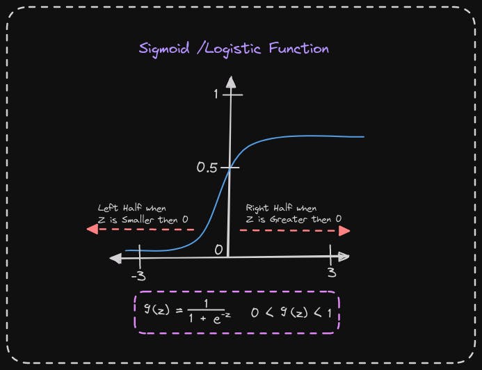
Whenever the value of z is greater than or equal to 0, the value of g(z) becomes greater than or equal to 0.5. This means that z must be on the right half of the axis. To determine when z is greater than or equal to zero, we should consider the formula z = w.x + b. Therefore, z is greater than or equal to zero if w.x + b is greater than or equal to zero.
To summarize, this model predicts 1 when w.x + b is greater than or equal to 0, and it predicts 0 when w.x + b is less than zero.
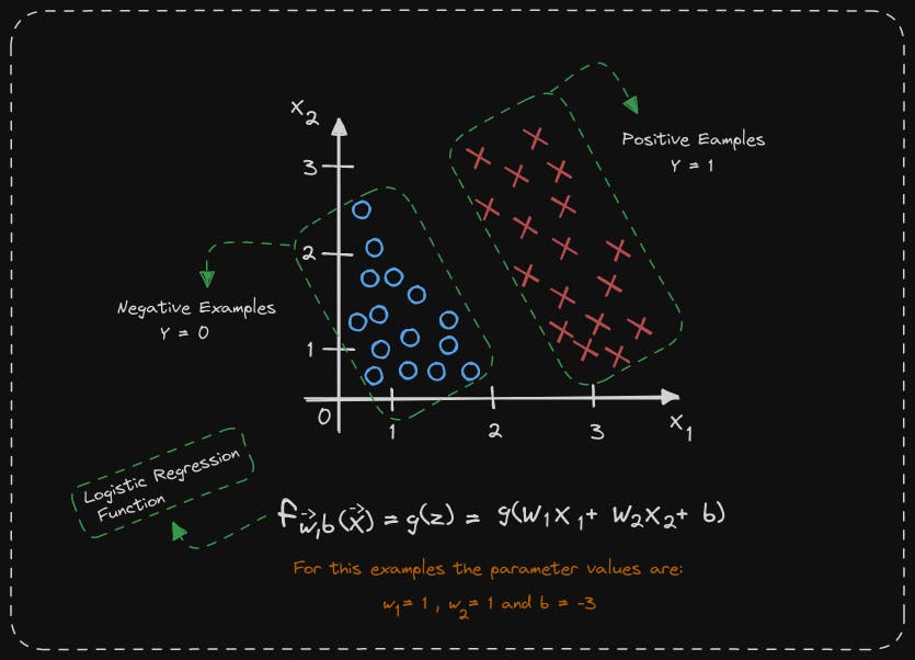
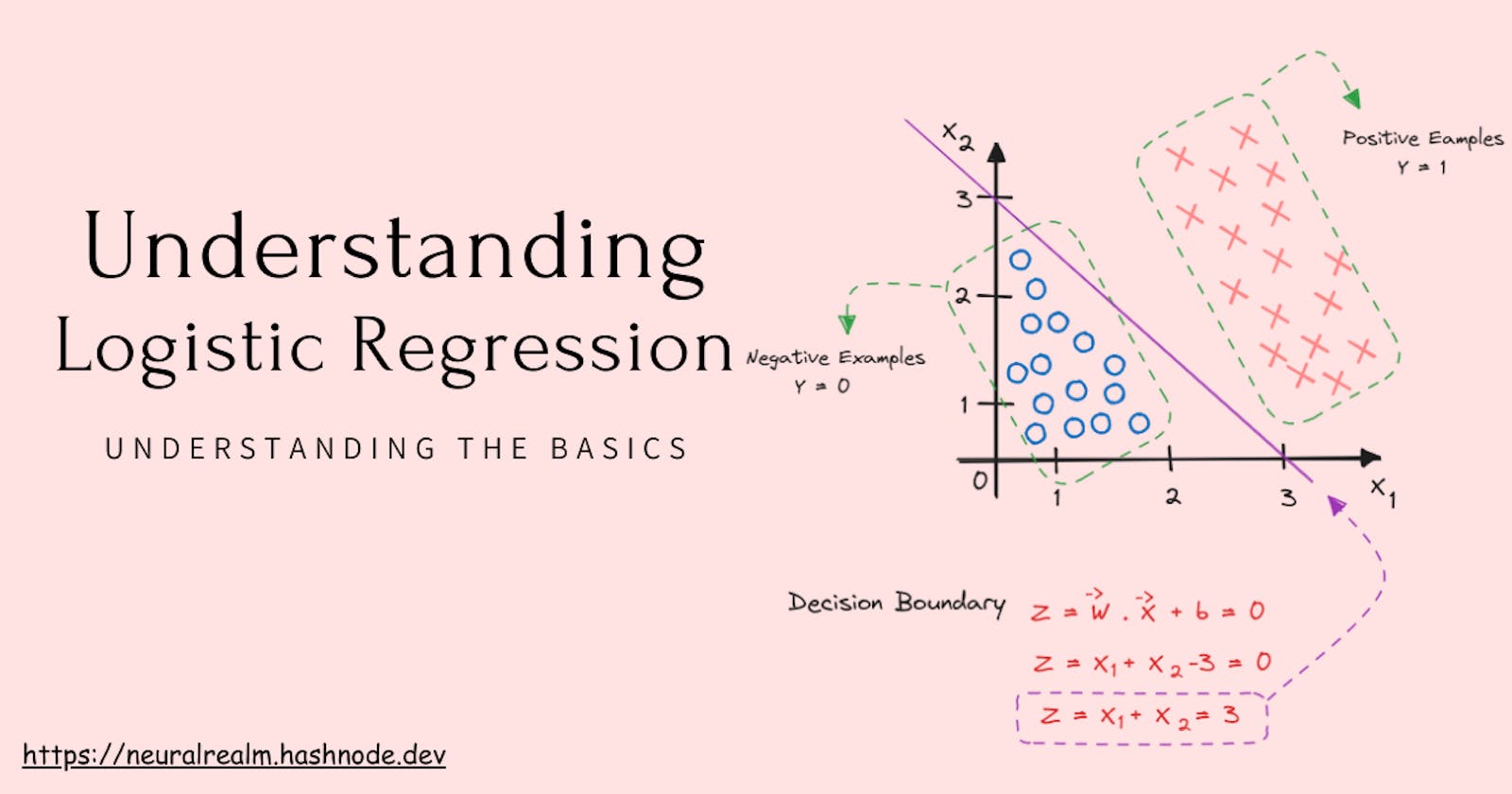
Let's examine how the model generates predictions by visualization. To illustrate this, consider a classification problem with two features, x1 and x2, instead of just one feature. We have a training set where the positive examples are represented by little red crosses and the negative examples are represented by little blue circles. The red crosses indicate y equals 1, while the blue circles correspond to y equals 0. The logistic regression model will use the function f of x equals g of z to make predictions. In this case, z is the expression w1x1 plus w2x2 plus b since we have two features x1 and x2. Let's assume that the parameter values for this example are w1 equals 1, w2 equals 1, and b equals negative 3.
Let's analyze how logistic regression predicts by determining when wx plus b is greater than or equal to 0 and when it's less than 0.
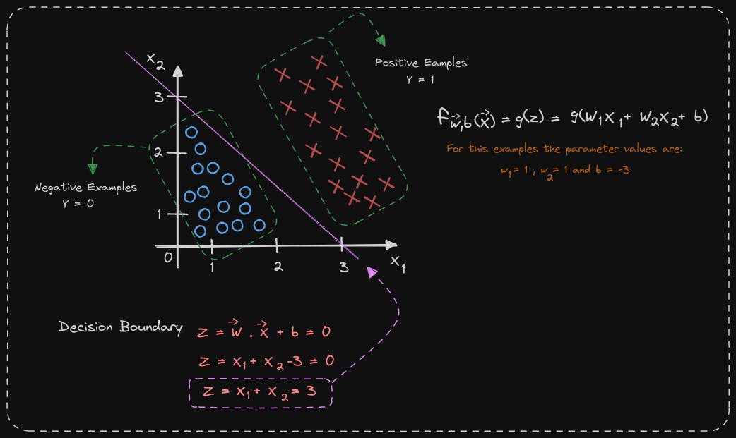
To determine a decision boundary, we look at the line where wx plus b equals 0. This line indicates the point at which we are almost neutral about whether y is 0 or 1. In our example, the decision boundary is x1 plus x2 minus 3, which corresponds to the line x1 plus x2 equals 3. This line serves as the decision boundary for logistic regression, predicting 1 for features to the right of the line and 0 for features to the left of the line. The parameters w1, w2, and b in our example are 1, 1, and -3, respectively. If we had different parameter values, the decision boundary would be a different line.
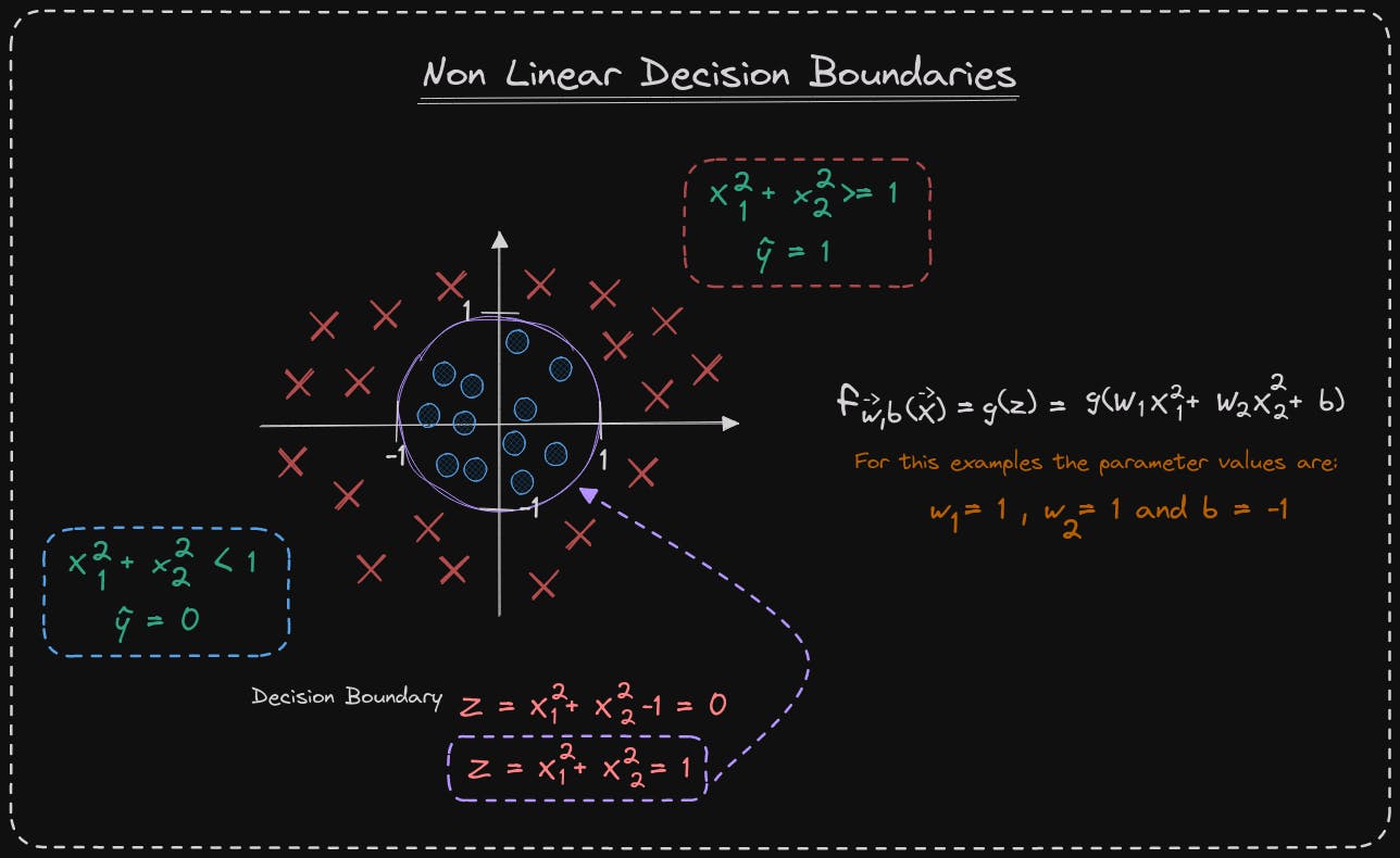
Let's consider a more complex example where the decision boundary is not a straight line. The cross symbol represents class y equals 1, and the little circle symbol denotes class y equals 0. Last week, you learned how to use polynomials in linear regression, and you can use them in logistic regression as well. We set z to be w_1, x_1 squared plus w_2, x_2 squared plus b, with this choice of features, we incorporate polynomial features into a logistic regression. The function f of x, which is equal to g of z, is now g of this expression over here. Suppose we choose w_1 and w_2 to be 1 and b to be negative 1. Then, z is equal to 1 times x_1 squared plus 1 times x_2 squared minus 1. The decision boundary, as before, corresponds to when z is equal to 0. This expression equals 0 when x_1 squared plus x_2 squared equals 1. If we plot the diagram on the left, the curve corresponding to x_1 squared plus x_2 squared equals 1 is the circle. When x_1 squared plus x_2 squared is greater than or equal to 1, that's the area outside the circle, and we predict y to be 1. Conversely, when x_1 squared plus x_2 squared is less than 1, that's the area inside the circle, and we predict y to be 0.
It is possible to create more complex decision boundaries by using higher-order polynomial terms.
Logistic regression is capable of fitting complex data by learning from it. However, if you exclude higher-order polynomials and only use features like x_1, x_2, x_3, etc., the decision boundary for logistic regression will always be a straight line and remain linear.
To gain a better understanding of how this process works, I recommend referring to this Notebook: Decision Boundary Notebook
🎙️ Message for Next Episode:
Now that you have an understanding of what function f(x) can potentially calculate, let's focus on how to train a logistic regression model. We will start by analyzing the cost function for logistic regression and then learn how to apply gradient descent to it. Let's proceed to the next episode.
Resources For Further Research
Coursera - Machine Learning Specialization
This Article is heavily inspired by this Course so I will also recommend you to check this course out, there is an option to watch the course for free.
"Hands-On Machine Learning with Scikit-Learn, Keras, and TensorFlow" by Aurélien Géron:
- A practical guide covering various machine learning concepts and implementations.
By the way…
Call to action
Hi, Everydaycodings— I’m building a newsletter that covers deep topics in the space of engineering. If that sounds interesting, subscribe and don’t miss anything. If you have some thoughts you’d like to share or a topic suggestion, reach out to me via LinkedIn or X(Twitter).
References
And if you’re interested in diving deeper into these concepts, here are some great starting points:
Kaggle Stories - Each episode of Kaggle Stories takes you on a journey behind the scenes of a Kaggle notebook project, breaking down tech stuff into simple stories.
Machine Learning - This series covers ML fundamentals & techniques to apply ML to solve real-world problems using Python & real datasets while highlighting best practices & limits.