


Recap from Previous Episodes
In the previous episodes, we discussed the basics of linear regression and differentiated between simple and multiple linear regression. Simple linear regression, which is expressed as y=mx+b, is used to model the connection between a dependent variable and a single independent variable, while multiple linear regression is used when we have more than one predictor variable. We looked at the mathematical formulas used, with a focus on the least squares method to obtain optimal coefficients. In Episode 8, we will now shift our focus to the practical application of linear regression. We will discuss data preparation, model building, and interpretation. Let's put our knowledge into practice and apply linear regression in real-world scenarios.
Importance of Practical Implementation
The practical implementation of linear regression is crucial for several reasons:
Validation of Theory:
- Validates theoretical concepts in real-world scenarios, ensuring the accuracy of the learned principles.
Hands-on Learning:
- It provides a hands-on learning experience, allowing practitioners to navigate challenges and develop practical skills.
Data Quality Insights:
- Exposes individuals to real-world data complexities, enhancing skills in data preprocessing and ensuring model training on high-quality data.
Model Evaluation and Tuning:
- Shifts focus to model evaluation, teaching practitioners how to assess performance and fine-tune models based on actual outcomes.
Decision-Making in Uncertainty:
- Equips individuals to make informed decisions in uncertain environments, considering the limitations and uncertainties associated with predictions.
Business Relevance:
- Enhances relevance in business and industry by providing practical solutions to real-world problems in various domains.
Communication Skills:
- Enables effective communication with non-technical stakeholders, translating technical results into actionable insights.
Continuous Improvement:
- Promotes a continuous improvement mindset, allowing for model adaptation to changing circumstances and evolving datasets.
Problem-Solving Skills:
- Hones problem-solving skills by presenting real challenges and encouraging effective solutions using linear regression.
Preparation for Advanced Concepts:
- Serves as a foundation for tackling more advanced concepts in machine learning and data science.
Practical implementation transforms theoretical knowledge into actionable insights, empowering individuals to make informed decisions and solve real-world problems.
Getting The Data
For the demonstration in this article, we will be using a dataset from Kaggle. Follow these Links to download the data:
https://www.kaggle.com/datasets/mirichoi0218/insurance
Data First Look
import pandas as pd
import numpy as np

data = pd.read_csv("/kaggle/input/insurance/insurance.csv")
data.head()
| age | sex | bmi | children | smoker | region | charges |
| 19 | female | 27.900 | 0 | yes | southwest | 16884.92400 |
| 18 | male | 33.770 | 1 | no | southeast | 1725.55230 |
| 28 | male | 33.000 | 3 | no | southeast | 4449.46200 |
| 33 | male | 22.705 | 0 | no | northwest | 21984.47061 |
| 32 | male | 28.880 | 0 | no | northwest | 3866.85520 |
data.info()
<class 'pandas.core.frame.DataFrame'>
RangeIndex: 1338 entries, 0 to 1337
Data columns (total 7 columns):
 #   Column    Non-Null Count  Dtype
---  ------    --------------  -----
 0   age       1338 non-null   int64
 1   sex       1338 non-null   object
 2   bmi       1338 non-null   float64
 3   children  1338 non-null   int64
 4   smoker    1338 non-null   object
 5   region    1338 non-null   object
 6   charges   1338 non-null   float64
dtypes: float64(2), int64(2), object(3)
memory usage: 73.3+ KB
Handling Missing Values
Dealing with missing data is crucial for robust model performance. It is important to consider imputation methods, as well as deciding whether to exclude or interpolate missing values based on the context.
data.isnull().sum()
age         0
sex         0
bmi         0
children    0
smoker      0
region      0
charges     0
dtype: int64
Fortunately, we do not have any null values in our data, which makes our work easier. However, it is not uncommon to encounter missing or null values in other data sets. Therefore, I am also creating code to handle such situations in case you are working with a different type of data.
"""Here are some common techniques to handle null values
   in Pandas"""

# Droping Null Values
data.dropna(inplace=True)

# Fill null values with the mean of the column
data.fillna(df.mean(), inplace=True)

# Or fill with a custom value
data.fillna(value=0, inplace=True)

# Linear interpolation
data.interpolate(method='linear', inplace=True)

# For Categorical Columns
data['categorical_column'].fillna(data['categorical_column'].mode()[0], inplace=True)
Distribution of values in Categorical columns
data["sex"].value_counts()
sex
male      676
female    662
Name: count, dtype: int64
data["smoker"].value_counts()
smoker
no     1064
yes     274
Name: count, dtype: int64
data["region"].value_counts()
region
southeast    364
southwest    325
northwest    325
northeast    324
Name: count, dtype: int64
The purpose of checking the distribution of the dataset was to ensure that there were no unusual occurrences in the data. For instance, in the sex column, we wanted to ensure that there were only male and female categories and no other unusual ones. Fortunately, we did not find any unusual occurrences, which is a good thing.
Changing the datatype
data["bmi"] = data["bmi"].astype(int)
data["charges"] = data["charges"].astype(int)
data.info()
<class 'pandas.core.frame.DataFrame'>
RangeIndex: 1338 entries, 0 to 1337
Data columns (total 7 columns):
 #   Column    Non-Null Count  Dtype
---  ------    --------------  -----
 0   age       1338 non-null   int64
 1   sex       1338 non-null   object
 2   bmi       1338 non-null   int64
 3   children  1338 non-null   int64
 4   smoker    1338 non-null   object
 5   region    1338 non-null   object
 6   charges   1338 non-null   int64
dtypes: int64(4), object(3)
memory usage: 73.3+ KB
we have changed bmi, charges from object to int64.
Splitting the Data
from sklearn.model_selection import train_test_split
X_train, X_test, y_train, y_test = train_test_split(data.drop('charges', axis=1),
                                                    data['charges'],
                                                    test_size=0.2,
                                                    random_state=0)

X_train.shape, X_test.shape
((1070, 6), (268, 6))
Feature Engineering
One Hot Encoding
One hot encoding is a technique that we use to represent categorical variables as numerical values in a machine learning model**.**
The advantages of using one hot encoding include:
It allows the use of categorical variables in models that require numerical input.
It can improve model performance by providing more information to the model about the categorical variable.
It can help to avoid the problem of ordinality, which can occur when a categorical variable has a natural ordering (e.g. “small”, “medium”, “large”).
The disadvantages of using one hot encoding include:
It can lead to increased dimensionality, as a separate column is created for each category in the variable. This can make the model more complex and slow to train.
It can lead to sparse data, as most observations will have a value of 0 in most of the one-hot encoded columns.
It can lead to overfitting, especially if there are many categories in the variable and the sample size is relatively small.
One-hot-encoding is a powerful technique to treat categorical data, but it can lead to increased dimensionality, sparsity, and overfitting. It is important to use it cautiously and consider other methods such as ordinal encoding or binary encoding.
import pandas as pd
from sklearn.preprocessing import OneHotEncoder
import numpy as np

cat_columns = ['sex', 'smoker', 'region']

ohe = OneHotEncoder(drop='first', sparse=False, dtype=np.int32)
X_train_encoded = ohe.fit_transform(X_train[cat_columns])
X_test_encoded = ohe.transform(X_test[cat_columns])

# Assuming X_train and X_test contain both numerical and categorical features
# X_train_numerical and X_test_numerical are the numerical features
X_train_numerical = X_train.drop(cat_columns, axis=1)
X_test_numerical = X_test.drop(cat_columns, axis=1)

# Convert NumPy arrays to DataFrames
X_train_numerical = pd.DataFrame(X_train_numerical, columns=X_train_numerical.columns)
X_test_numerical = pd.DataFrame(X_test_numerical, columns=X_test_numerical.columns)

# Concatenate the numerical features with the encoded categorical features
X_train_encoded = pd.concat([X_train_numerical, pd.DataFrame(X_train_encoded, columns=ohe.get_feature_names_out(cat_columns))], axis=1)
X_test_encoded = pd.concat([X_test_numerical, pd.DataFrame(X_test_encoded, columns=ohe.get_feature_names_out(cat_columns))], axis=1)
X_train_encoded
| age | bmi | children | sex_male | smoker_yes | region_northwest | region_southeast | region_southwest |
| 37.0 | 34.0 | 4.0 | 1.0 | 1.0 | 0.0 | 0.0 | 1.0 |
| 18.0 | 34.0 | 0.0 | 1.0 | 0.0 | 0.0 | 1.0 | 0.0 |
| 23.0 | 36.0 | 2.0 | 1.0 | 0.0 | 1.0 | 0.0 | 0.0 |
| 32.0 | 35.0 | 2.0 | NaN | NaN | NaN | NaN | NaN |
| 58.0 | 32.0 | 1.0 | NaN | NaN | NaN | NaN | NaN |
| ... | ... | ... | ... | ... | ... | ... | ... |
| NaN | NaN | NaN | 1.0 | 0.0 | 1.0 | 0.0 | 0.0 |
| NaN | NaN | NaN | 0.0 | 0.0 | 1.0 | 0.0 | 0.0 |
| NaN | NaN | NaN | 0.0 | 0.0 | 0.0 | 0.0 | 1.0 |
| NaN | NaN | NaN | 0.0 | 0.0 | 0.0 | 0.0 | 1.0 |
| NaN | NaN | NaN | 0.0 | 0.0 | 1.0 | 0.0 | 0.0 |
Feature Scaling
What is Feature Scaling?
Feature Scaling is a technique to standardize the independent features present in the data in a fixed range. It is performed during the data pre-processing to handle highly varying magnitudes or values or units. If feature scaling is not done, then a machine learning algorithm tends to weigh greater values, higher and consider smaller values as the lower values, regardless of the unit of the values.
Why use Feature Scaling?
In machine learning, feature scaling is employed for a number of purposes:
Scaling guarantees that all features are on a comparable scale and have comparable ranges. This process is known as feature normalization. This is significant because the magnitude of the features has an impact on many machine-learning techniques. Larger scale features may dominate the learning process and have an excessive impact on the outcomes. You can avoid this problem and make sure that each feature contributes equally to the learning process by scaling the features.
Algorithm performance improvement: When the features are scaled, several machine learning methods, including gradient descent-based algorithms, distance-based algorithms (such k-nearest neighbours), and support vector machines, perform better or converge more quickly. The algorithm’s performance can be enhanced by scaling the features, which can hasten the convergence of the algorithm to the ideal outcome.
Preventing numerical instability: Numerical instability can be prevented by avoiding significant scale disparities between features. Examples include distance calculations or matrix operations, where having features with radically differing scales can result in numerical overflow or underflow problems. Stable computations are ensured and these issues are mitigated by scaling the features.
Scaling features ensure that each characteristic is given the same consideration during the learning process. Without scaling, bigger scale features could dominate the learning, producing skewed outcomes. This bias is removed through scaling, which also guarantees that each feature contributes fairly to model predictions.
What is Normalization?
Normalization is a data preprocessing technique used to adjust the values of features in a dataset to a common scale. This is done to facilitate data analysis and modeling and to reduce the impact of different scales on the accuracy of machine learning models.
Normalization is a scaling technique in which values are shifted and rescaled so that they end up ranging between 0 and 1. It is also known as Min-Max scaling.

Here, Xmax and Xmin are the maximum and the minimum values of the feature, respectively.
When the value of X is the minimum value in the column, the numerator will be 0, and hence X’ is 0
On the other hand, when the value of X is the maximum value in the column, the numerator is equal to the denominator, and thus the value of X’ is 1
If the value of X is between the minimum and the maximum value, then the value of X’ is between 0 and 1
What is Standardization?
Standardization is another scaling method where the values are centered around the mean with a unit standard deviation. This means that the mean of the attribute becomes zero, and the resultant distribution has a unit standard deviation.
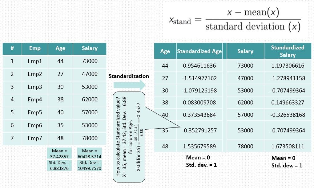
Mu is the mean of the feature values and Sigma is the standard deviation of the feature values. Note that, in this case, the values are not restricted to a particular range.
The Big Question – Normalize or Standardize?
Normalization:
Purpose: Rescales values to a range between 0 and 1.
When to use: Useful when the distribution of the data is unknown or not Gaussian.
Sensitivity to outliers: Sensitive to outliers.
Shape of distribution: Retains the shape of the original distribution.
Preservation of relationships: May not preserve the relationships between the data points.
Equation:
$$\frac{x - \text{min}}{\text{max} - \text{min}}$$
Standardization:
Purpose: Centers data around the mean and scales to a standard deviation of 1.
When to use: Useful when the distribution of the data is Gaussian or unknown.
Sensitivity to outliers: Less sensitive to outliers.
Shape of distribution: Changes the shape of the original distribution.
Preservation of relationships: Preserves the relationships between the data points.
Equation:
$$\frac{x - \text{mean}}{\text{standard deviation}}$$
from sklearn.preprocessing import StandardScaler

scaler = StandardScaler()

# fit the scaler to the train set, it will learn the parameters
scaler.fit(X_train_encoded)

# transform train and test sets
X_train_scaled = scaler.transform(X_train_encoded)
X_test_scaled = scaler.transform(X_test_encoded)
X_train_scaled
array([[-0.14853305,  0.60616004,  2.41394802, ..., -0.55791981,
        -0.6155209 ,  1.70862925],
       [-1.49780784,  0.60616004, -0.89219519, ..., -0.55791981,
         1.6246402 , -0.58526447],
       [-1.14273553,  0.92836135,  0.76087642, ...,  1.79237229,
        -0.6155209 , -0.58526447],
       ...,
       [        nan,         nan,         nan, ..., -0.55791981,
        -0.6155209 ,  1.70862925],
       [        nan,         nan,         nan, ..., -0.55791981,
        -0.6155209 ,  1.70862925],
       [        nan,         nan,         nan, ...,  1.79237229,
        -0.6155209 , -0.58526447]])
X_train_scaled = pd.DataFrame(X_train_scaled, columns=X_train_encoded.columns)
X_test_scaled = pd.DataFrame(X_test_scaled, columns=X_test_encoded.columns)
I plot a graph to compare the data before and after feature scaling to see the differences.
import matplotlib.pyplot as plt
import seaborn as sns

# Assuming X_train contains 'age', 'bmi', 'children' columns
# and X_train_scaled contains the scaled values of these columns

fig, axes = plt.subplots(nrows=2, ncols=2, figsize=(15, 10))

# Scatter plot for 'age' and 'bmi' before scaling
axes[0, 0].scatter(X_train['age'], X_train['bmi'], color='red')
axes[0, 0].set_title("Before Scaling")
axes[0, 0].set_xlabel('Age')
axes[0, 0].set_ylabel('BMI')

# Scatter plot for 'age' and 'bmi' after scaling
axes[0, 1].scatter(X_train_scaled['age'], X_train_scaled['bmi'], color='red')
axes[0, 1].set_title("After Scaling")
axes[0, 1].set_xlabel('Scaled Age')
axes[0, 1].set_ylabel('Scaled BMI')

# Scatter plot for 'children' and 'bmi' before scaling
axes[1, 0].scatter(X_train['children'], X_train['bmi'], color='green')
axes[1, 0].set_title("Before Scaling")
axes[1, 0].set_xlabel('Children')
axes[1, 0].set_ylabel('BMI')

# Scatter plot for 'children' and 'bmi' before scaling
axes[1, 1].scatter(X_train_scaled['children'], X_train_scaled['bmi'], color='green')
axes[1, 1].set_title("Before Scaling")
axes[1, 1].set_xlabel('Children')
axes[1, 1].set_ylabel('BMI')

plt.tight_layout()
plt.show()

When Feature Scaling is applied, there is no difference in shape. This is attributed to +point.
Using Pipeline
Explanation of why using a pipeline is beneficial compared to applying preprocessing steps separately
Readability and Convenience:
Pipelines provide a clean and readable way to organize the entire workflow in a single object.
It simplifies the code and makes it easy to understand the sequence of operations.
Data Leakage Prevention:
Pipelines automatically handle data leakage, ensuring that preprocessing steps are applied consistently to both training and test sets.
This reduces the risk of unintentionally incorporating information from the test set into the training process.
Consistency and Error Reduction:
- Pipelines ensure consistent application of preprocessing steps, reducing the chance of errors that might occur when applying transformations separately.
Easier Deployment:
- When deploying machine learning models, pipelines make it straightforward to apply the same preprocessing steps to new data consistently.
Integration with Hyperparameter Tuning:
Pipelines seamlessly integrate with hyperparameter tuning tools like Grid Search.
This simplifies the optimization process for both preprocessing and modeling steps.
Code Reproducibility:
Pipelines contribute to code reproducibility by encapsulating the entire workflow in a single object.
This makes it easier to share and reproduce results.
Pipeline for OneHotEncoder and StandardScaler
from sklearn.compose import ColumnTransformer
from sklearn.pipeline import Pipeline
from sklearn.preprocessing import StandardScaler, OneHotEncoder
from sklearn.linear_model import LinearRegression

# Assuming you have a DataFrame X_train with columns 'age', 'bmi', 'children', and 'charges'
numerical_features = ['age', 'bmi', 'children']
categorical_features = ['sex', 'smoker', 'region']

# Create transformers for numerical and categorical features
numerical_transformer = StandardScaler()
categorical_transformer = OneHotEncoder(drop='first', sparse_output=False, dtype=int)

# Create a column transformer to apply transformers to the respective feature groups
preprocessor = ColumnTransformer(
    transformers=[
        ('num', numerical_transformer, numerical_features),
        ('cat', categorical_transformer, categorical_features)
    ])
pipeline = Pipeline(steps=[('preprocessor', preprocessor)])

# Fit and transform the training data
X_train_transformed = pipeline.fit_transform(X_train)

# Transform the test data (using the learned parameters from the training data)
X_test_transformed = pipeline.transform(X_test)
In this example, fit_transform is used on the training data (X_train), and then transform is used on the test data (X_test). This ensures that the same scaling parameters learned from the training data are applied to both sets consistently.
In summary, use fit_transform on the training data to learn parameters and transform it, and then use transform on new data using the same transformer to apply the learned parameters.
Model Creation
Linear Regression
from sklearn.compose import ColumnTransformer
from sklearn.pipeline import Pipeline
from sklearn.preprocessing import StandardScaler, OneHotEncoder
from sklearn.linear_model import LinearRegression
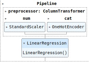
# Create the pipeline with a model (Linear Regression in this case) as the final step
linear_pipeline = Pipeline(steps=[
('preprocessor', preprocessor),
('regressor', LinearRegression())
])
# Fit the pipeline on the training data
linear_pipeline.fit(X_train, y_train)
# Make predictions on the test data
linear_predictions = linear_pipeline.predict(X_test)
linear_pipeline
Regression Metrics
Mean Absolute Error (MAE):
Measures the average absolute difference between the predicted and actual values.
$$MAE = \frac{1}{n} \sum_{i=1}^{n} \left| y_i - \hat{y}_i \right|$$
Mean Squared Error (MSE):
Measures the average squared difference between the predicted and actual values.
$$MSE = \frac{1}{n} \sum_{i=1}^{n} (y_i - \hat{y}_i)^2$$
Root Mean Squared Error (RMSE):
The square root of the MSE. It provides an interpretable measure in the same units as the target variable.
$$RMSE = \sqrt{MSE}$$
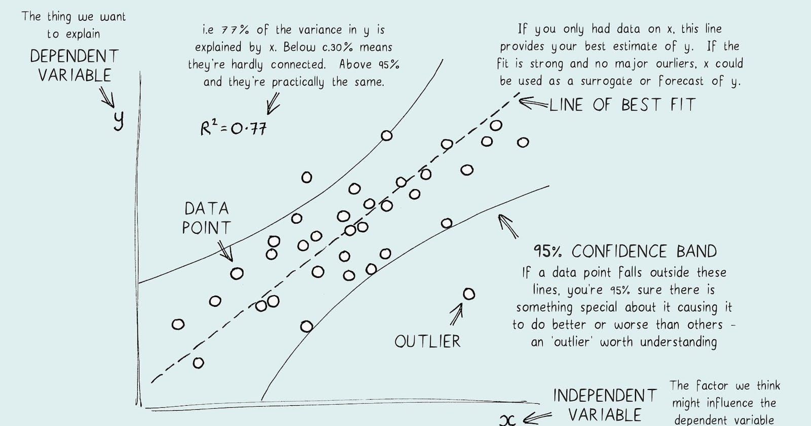
R-squared (R2) Score:
Measures the proportion of the variance in the dependent variable that is predictable from the independent variables.
$$R^2 = 1 - \frac{\sum_{i=1}^{n} (y_i - \hat{y}i)^2}{\sum{i=1}^{n} (y_i - \bar{y})^2}$$
from sklearn.metrics import mean_absolute_error, mean_squared_error, r2_score

# Assuming 'predictions' contains the predicted values
# and 'y_test' contains the true values in the test set

# Mean Absolute Error
linear_mae = mean_absolute_error(y_test, linear_predictions)

# Mean Squared Error
linear_mse = mean_squared_error(y_test, linear_predictions)

# Root Mean Squared Error
linear_rmse = np.sqrt(linear_mse)

# R-squared (R2) Score
linear_r2 = r2_score(y_test, linear_predictions)

print(f'Mean Absolute Error: {linear_mae}')
print(f'Mean Squared Error: {linear_mse}')
print(f'Root Mean Squared Error: {linear_rmse}')
print(f'R-squared Score: {linear_r2}')
Mean Absolute Error: 3925.5806672697704
Mean Squared Error: 31893147.45437684
Root Mean Squared Error: 5647.401832203623
R-squared Score: 0.7995787849960009
Lower MAE, MSE, and RMSE values indicate better model performance, as they represent smaller prediction errors.
A higher R2 score (closer to 1) indicates a better model fit, with a higher proportion of variance explained by the model.
GridSearchCV
GridSearchCV is a module in scikit-learn that provides an exhaustive search over a specified parameter grid to find the best combination of hyperparameters for a machine learning model. It performs cross-validated grid search, meaning it evaluates the performance of the model with different hyperparameter combinations using cross-validation.
Here's a brief overview of the main components and functionality of GridSearchCV:
Parameter Grid: You define a grid of hyperparameter values that you want to search over. For each combination of hyperparameters in the grid, GridSearchCV trains the model and evaluates its performance.
Cross-Validation: GridSearchCV performs k-fold cross-validation for each set of hyperparameters. It divides the training data into k folds, trains the model on k-1 folds, and evaluates it on the remaining fold. This process is repeated k times, and the performance is averaged.
Scoring: You specify a scoring metric to evaluate the performance of the model for each combination of hyperparameters. Common metrics for regression tasks include Mean Squared Error ('neg_mean_squared_error') or R-squared ('r2').
Parallelization: GridSearchCV can run the grid search in parallel, taking advantage of multiple CPU cores, which can significantly speed up the search process.
Best Model and Best Parameters: After the search, GridSearchCV provides the best hyperparameters and the corresponding model, which can be used for making predictions on new data.
Lasso Regression
from sklearn.model_selection import GridSearchCV
from sklearn.linear_model import Lasso, Ridge

# Create a pipeline with a model (Lasso Regression) as the final step
lasso_pipeline = Pipeline(steps=[
    ('preprocessor', preprocessor),
    ('regressor', Lasso())
])

# Create a parameter grid to search for Lasso Regression
lasso_param_grid = {
    'regressor__alpha': [0.1, 1.0, 10.0],
    'regressor__selection': ['cyclic', 'random']
    # Add other hyperparameters to tune
}

# Create the GridSearchCV object for Lasso Regression
lasso_grid_search = GridSearchCV(lasso_pipeline, lasso_param_grid, cv=5, scoring='neg_mean_squared_error', n_jobs=-1)

# Fit the grid search to the data for Lasso Regression
lasso_grid_search.fit(X_train, y_train)

# Make predictions on the test data
lasso_predictions = lasso_grid_search.predict(X_test)

# Get the best hyperparameters for Lasso Regression
best_lasso_params = lasso_grid_search.best_params_

# Get the best model for Lasso Regression
best_lasso_model = lasso_grid_search.best_estimator_
# Mean Absolute Error
lasso_mae = mean_absolute_error(y_test, lasso_predictions)

# Mean Squared Error
lasso_mse = mean_squared_error(y_test, lasso_predictions)

# Root Mean Squared Error
lasso_rmse = np.sqrt(lasso_mse)

# R-squared (R2) Score
lasso_r2 = r2_score(y_test, lasso_predictions)

print(f'Mean Absolute Error: {lasso_mae}')
print(f'Mean Squared Error: {lasso_mse}')
print(f'Root Mean Squared Error: {lasso_rmse}')
print(f'R-squared Score: {lasso_r2}')
Mean Absolute Error: 3934.6211207137017
Mean Squared Error: 31978089.926188666
Root Mean Squared Error: 5654.917322666059
R-squared Score: 0.7990449940482645
Ridge Regression
ridge_pipeline = Pipeline(steps=[
    ('preprocessor', preprocessor),
    ('regressor', Ridge())
])

ridge_param_grid = {
    'regressor__alpha': [0.1, 1.0, 10.0],
    'regressor__solver': ['auto', 'svd', 'cholesky', 'lsqr', 'sparse_cg', 'sag', 'saga', 'lbfgs']
    # Add other hyperparameters to tune
}

ridge_grid_search = GridSearchCV(ridge_pipeline, ridge_param_grid, cv=5, scoring='neg_mean_squared_error', n_jobs=-1)
ridge_grid_search.fit(X_train, y_train)
ridge_predictions = ridge_grid_search.predict(X_test)

best_ridge_params = ridge_grid_search.best_params_
best_ridge_model = ridge_grid_search.best_estimator_
# Mean Absolute Error
ridge_mae = mean_absolute_error(y_test, ridge_predictions)

# Mean Squared Error
ridge_mse = mean_squared_error(y_test, ridge_predictions)

# Root Mean Squared Error
ridge_rmse = np.sqrt(ridge_mse)

# R-squared (R2) Score
ridge_r2 = r2_score(y_test, ridge_predictions)

print(f'Mean Absolute Error: {ridge_mae}')
print(f'Mean Squared Error: {ridge_mse}')
print(f'Root Mean Squared Error: {ridge_rmse}')
print(f'R-squared Score: {ridge_r2}')
Mean Absolute Error: 3927.1989340915807
Mean Squared Error: 31899299.199522503
Root Mean Squared Error: 5647.9464586274635
R-squared Score: 0.7995401265274927
Final Look
metrics_df = pd.DataFrame({
    'Model': ['Linear Regression', 'Lasso Regression', 'Ridge Regression'],
    'MSE': [linear_mse,lasso_mse,ridge_mse],
    'MAE': [linear_mae,lasso_mae,ridge_mae],
    'RMSE': [linear_rmse,lasso_rmse,ridge_rmse],
    'R2': [linear_r2,lasso_r2,ridge_r2]
})

# Display the DataFrame
metrics_df
| Model | MSE | MAE | RMSE | R2 |
| Linear Regression | 3.189315e+07 | 3925.580667 | 5647.401832 | 0.799579 |
| Lasso Regression | 3.197809e+07 | 3934.621121 | 5654.917323 | 0.799045 |
| Ridge Regression | 3.189930e+07 | 3927.198934 | 5647.946459 | 0.799540 |
Practical Tips for Success
Successfully implementing linear regression involves more than just writing code. Consider the following practical tips to enhance your success in applying linear regression models:
Understand Your Data Domain
Before diving into modeling, thoroughly understand the domain of your data. Knowing the context helps in selecting relevant features, interpreting results, and making informed decisions.
Feature Engineering
Explore and create meaningful features that can enhance the model's predictive power. This involves transforming existing features or creating new ones based on domain knowledge.
Regularly Check Assumptions
Linear regression relies on certain assumptions. Regularly check for violations, such as linearity, independence, and homoscedasticity. Addressing these issues ensures the reliability of your model.
Optimize Hyperparameters
Experiment with different hyperparameters to optimize model performance. This includes adjusting regularization parameters for better generalization to new data.
Handle Multicollinearity
Detect and address multicollinearity among predictor variables. A high correlation between features can lead to instability in coefficient estimates. Consider techniques like variance inflation factor (VIF) analysis.
Robustness to Outliers
Be mindful of outliers' impact on the model. Consider using robust regression techniques or transforming variables to minimize the influence of extreme values.
Interpretability Matters
Ensure your model is interpretable, especially if you need to explain results to non-technical stakeholders. Clearly communicate the meaning of coefficients in the context of your problem.
Cross-Validate Religiously
Use cross-validation techniques extensively to assess your model's generalization performance. This helps in identifying potential issues like overfitting and ensures your model is robust.
Stay Updated on Industry Practices
Keep yourself informed about the latest practices and advancements in linear regression and related fields. Staying updated ensures you can leverage the most effective techniques for your projects.
Document Your Process
Maintain clear documentation of your data preprocessing steps, model choices, and results interpretation. A well-documented process aids reproducibility and facilitates collaboration with colleagues.
By incorporating these practical tips into your linear regression implementation, you'll be better equipped to handle real-world challenges and achieve more accurate and meaningful results.
Conclusion
In this article, we explored linear regression from theory to implementation. We covered simple and multiple linear regression, data preparation, and practical tips for success. We also discussed strategies for enhancing model performance and interpreting results. The overall message is that linear regression is a powerful tool for making informed decisions. Remember to stay curious and embrace the continuous learning journey.
If you have an interest in the code, I have uploaded it on Kaggle. Here is the link:
https://www.kaggle.com/code/everydaycodings/understanding-linear-regression-from-scratch
🎙️ Message for Next Episode:
In the next episode, we'll delve into logistic regression - a powerful machine-learning algorithm for binary/categorical outcomes. Unlike linear regression, it maps input features into probabilities using the sigmoid function. We'll explain the concepts, showcase real-world applications, and demonstrate their effectiveness in solving practical problems. From predicting customer churn to identifying spam emails, logistic regression is an essential tool in machine learning. Join us on this educational journey to unlock its potential using Python. Don't miss out! 🚀🔍
Resources For Further Research
Coursera - Machine Learning Specialization
This Article is heavily inspired by this Course so I will also recommend you to check this course out, there is an option to watch the course for free.
"Hands-On Machine Learning with Scikit-Learn, Keras, and TensorFlow" by Aurélien Géron:
- A practical guide covering various machine learning concepts and implementations.
By the way…
Call to action
Hi, Everydaycodings— I’m building a newsletter that covers deep topics in the space of engineering. If that sounds interesting, subscribe and don’t miss anything. If you have some thoughts you’d like to share or a topic suggestion, reach out to me via LinkedIn or X.
References
And if you’re interested in diving deeper into these concepts, here are some great starting points:
Kaggle Stories - Each episode of Kaggle Stories takes you on a journey behind the scenes of a Kaggle notebook project, breaking down tech stuff into simple stories.
Machine Learning - This series covers ML fundamentals & techniques to apply ML to solve real-world problems using Python & real datasets while highlighting best practices & limits.